Climatological Means

In this tutorial, we’ll look at how to use wxee to calculate long-term climatological means of gridded weather data. Currently, monthly and daily mean climatologies are supported.

Setup

!pip install wxee

import ee
import wxee

ee.Authenticate()
wxee.Initialize()

Create a Time Series

Time-based methods in wxee, like temporal aggregation and climatology, work with the TimeSeries subclass of ee.ImageCollection. To use them, we’ll need to create a TimeSeries. There are two ways to do this.

From an Image Collection

Create an ee.ImageCollection and use the wx accessor and the to_time_series method to convert the Image Collection to a TimeSeries.

rtma = ee.ImageCollection("IDAHO_EPSCOR/GRIDMET")
ts = rtma.wx.to_time_series()

From Scratch

As a shortcut, you can create a TimeSeries just like you would create an ee.ImageCollection. Just pass a collection ID or list of Images.

ts = wxee.TimeSeries("IDAHO_EPSCOR/GRIDMET")

Monthly Total Rainfall

gridMET contains daily weather data including precipitation. First, we’ll load 10 years of data from 2000 - 2010 into a TimeSeries, giving us several thousand daily images.

ts = ts.select("pr")
ts = ts.filterDate("2000", "2010")

ts.size().getInfo()

3653

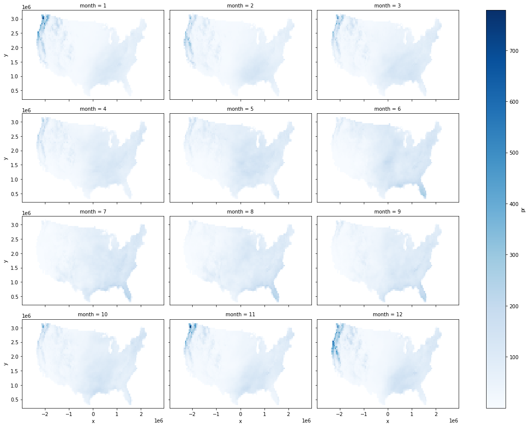
Now, we’ll calculate the monthly mean total rainfall over the 10 years, giving us just 12 images (one per month).

clim = ts.climatology_mean(frequency="month", reducer=ee.Reducer.sum())
clim.size().getInfo()

12

Tip: The reducer argument defines how data will be aggregated before the mean climatology is calculated. In this case, we’ll sum the daily precipitation to get monthly totals. The mean monthly climatology will be calculated from those totals.

Finally, we’ll download the monthly mean totals as an xarray dataset and plot them.

x = clim.wx.to_xarray(scale=50_000, crs="EPSG:5070")
x.pr.plot(col="month", col_wrap=3, figsize=(16, 12), cmap="Blues")

<xarray.plot.facetgrid.FacetGrid at 0x7f7945fc6dc0>

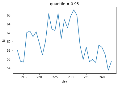
Daily Mean Burning Index

Once again we’ll look at gridMET daily weather data, but this time we’ll calculate the climatological mean burning index (a measure of wildfire potential) by day-of-year. Day-of-year climatologies require processing a lot more data, so we’ll just use 4 years for this example.

ts = wxee.TimeSeries("IDAHO_EPSCOR/GRIDMET").select("bi")
ts = ts.filterDate("2000", "2004")

A day-of-year climatology will give 366 images, one for each day through the 4 years (including leap days).

Note: Julian dates are used to calculate day-of-year means in wxee, so days after February 29 will be offset by one in leap years. For example, day-of-year 365 will represent December 31 in non-leap years and December 30 in leap years. Day 366 will always represent December 31, but will be aggregated from 1/4 as many days as other days of the year.

clim = ts.climatology_mean(frequency="day")
clim.size().getInfo()

366

We could download all 366 images, but maybe we’re only interested in burning index for the month of August. We can use the start and end args to set the climatological window of days to look at.

Here we’ll set the start to 213 and the end to 243 (Aug. 1 and Aug. 31 in non-leap years). Now we only have 31 images.

clim = ts.climatology_mean(frequency="day", start=213, end=243)
clim.size().getInfo()

31

Tip: Downloading is the slowest part of dealing with Earth Engine data in wxee, so it’s always best to aggregate and filter your data before downloading.

Let’s download them.

aug_bi = clim.wx.to_xarray(scale=50_000, crs="EPSG:5070")

And finally, we’ll plot a timeline of 95th percentile burning index values over the CONUS.

aug_bi.bi.quantile(0.95, ["x", "y"]).plot()

[<matplotlib.lines.Line2D at 0x7f7944057430>]

Note

This page was auto-generated from a Jupyter notebook. For full functionality, download the notebook from Github and run it in a local Python environment.