Climatological Anomalies

In this tutorial, we’ll look at how to use wxee to calculate long-term climatological anomalies with gridded weather data. Anomalies represent the difference between an observation and the long-term climatological mean for a given day or month.

Setup

!pip install wxee

import ee
import wxee

ee.Authenticate()
wxee.Initialize()

June 2021 Heat Wave

In late June of 2021, the Pacific Northwest of North America experienced an historic heat wave that broke many temperature records. Calculating monthly max temperature anomalies for this period will highlight just how unusual the observed weather was.

Reference and Observation Data

To start, we’ll load a TimeSeries of daily temperature data from gridMET.

temp = wxee.TimeSeries("IDAHO_EPSCOR/GRIDMET").select("tmmx")

Next, we’ll split our TimeSeries into two periods.

The first TimeSeries will be our 30-year reference period for calculating long-term climatological normals. We’ll use this as a baseline to identify anomalies during the heat wave.

ref = temp.filterDate("1980", "2010")

The second TimeSeries is our observation period, spanning about five months around the June heat wave.

obs = temp.filterDate("2021-04", "2021-09")

Climatological Mean

Now we can calculate the monthly climatological mean temperature over our reference period. We’ll use ee.Reducer.max() to get the maximum daily temperature in each month.

mean_clim = ref.climatology_mean("month", reducer=ee.Reducer.max())

Climatological Anomaly

Now we’ll calculate monthly temperature anomalies within our observation period based on the climatological means from our reference period.

The same frequency and reducer used in by mean_clim will be applied to the climatology anomaly.

anom = obs.climatology_anomaly(mean=mean_clim)

Download the data to an xarray.Dataset.

ds = anom.wx.to_xarray(crs="EPSG:5070", scale=20_000)

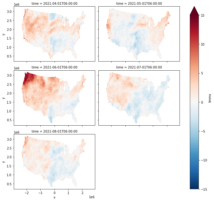
Plotting the monthly data, we can see that maximum temperatures in June in the Pacific Northwest exceeded long-term climatological normals by more than 15 °C!

ds.tmmx.plot(
    col="time", col_wrap=2, aspect=1.5,
    vmin=-15, vmax=15,
    cmap="RdBu_r"
)

<xarray.plot.facetgrid.FacetGrid at 0x7f1b8f490a60>

Standardized Anomalies

Standardized anomalies, which represent the number of standard deviations that an observation differed from the long-term mean, can also be calculated with wxee. Just calculate a long-term climatological standard deviation using TimeSeries.climatology_std and pass that to the std argument!

std_clim = ref.climatology_std("month", reducer=ee.Reducer.max())

std_anom = obs.climatology_anomaly(
    mean=mean_clim,
    std=std_clim,
)

Download to an xarray.Dataset.

std_ds = std_anom.wx.to_xarray(crs="EPSG:5070", scale=20_000)

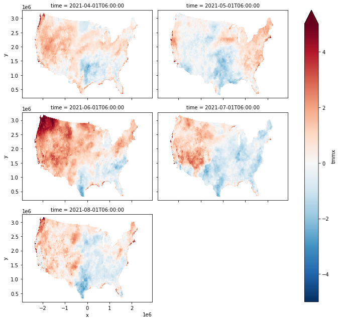
And plot! The data looks similar to above, but now we know that the ~15 °C anomalies that we saw above were more than 4 standard deviations hotter than the long-term mean!

std_ds.tmmx.plot(
    col="time", col_wrap=2, aspect=1.5,
    vmin=-5, vmax=5,
    cmap="RdBu_r"
)

<xarray.plot.facetgrid.FacetGrid at 0x7f1b8f57fc10>

Note

This page was auto-generated from a Jupyter notebook. For full functionality, download the notebook from Github and run it in a local Python environment.