![]()
![]()
Image Collection to xarray
In this tutorial, we’ll look at how we can use wxee and the wx accessor to convert an ee.ImageCollection of gridMET weather data to an xarray.Dataset for visualization and further processing.
Setup
[ ]:
!pip install wxee
[1]:
import ee
import wxee

ee.Authenticate()
wxee.Initialize()
Converting to xarray
Load the gridMET image collection.
[2]:
gridmet = ee.ImageCollection("IDAHO_EPSCOR/GRIDMET")
Select a date range of the collection to download to xarray. gridMET has 1 image per day, so this will give us 6 images.
[3]:
collection = gridmet.filterDate("2020-09-05", "2020-09-11")
Set the download parameters. We’ll use the full gridMET image extent of the continental US, but if we wanted to select a specific region we could pass an ee.Geometry.Polygon to the region argument.
[4]:
# The coordinate reference system to use (NAD83 Albers CONUS)
crs = "EPSG:5070"
# Spatial resolution in CRS units (meters)
scale = 20_000
The wx accessor extends images and image collections with additional functionality including to_xarray. We’ll use that to download the collection, storing it in memory as an xarray.Dataset.
[5]:
arr = collection.wx.to_xarray(scale=scale, crs=crs)
Tip: If the download fails due to a DownloadError, retry or increase the max_attempts argument.
The downloaded array has 6 time coordinates (1 for each image) and 16 variables (1 for each band).
[7]:
arr
[7]:
<xarray.Dataset>
Dimensions:  (time: 6, y: 154, x: 292)
Coordinates:
  * time     (time) datetime64[ns] 2020-09-05T06:00:00 ... 2020-09-10T06:00:00
  * y        (y) float64 3.27e+06 3.25e+06 3.23e+06 ... 2.5e+05 2.3e+05 2.1e+05
  * x        (x) float64 -2.91e+06 -2.89e+06 -2.87e+06 ... 2.89e+06 2.91e+06
Data variables: (12/16)
    pr       (time, y, x) float32 nan nan nan nan nan ... nan nan nan nan nan
    rmax     (time, y, x) float32 nan nan nan nan nan ... nan nan nan nan nan
    rmin     (time, y, x) float32 nan nan nan nan nan ... nan nan nan nan nan
    sph      (time, y, x) float32 nan nan nan nan nan ... nan nan nan nan nan
    srad     (time, y, x) float32 nan nan nan nan nan ... nan nan nan nan nan
    th       (time, y, x) float32 nan nan nan nan nan ... nan nan nan nan nan
    ...       ...
    eto      (time, y, x) float32 nan nan nan nan nan ... nan nan nan nan nan
    bi       (time, y, x) float32 nan nan nan nan nan ... nan nan nan nan nan
    fm100    (time, y, x) float32 nan nan nan nan nan ... nan nan nan nan nan
    fm1000   (time, y, x) float32 nan nan nan nan nan ... nan nan nan nan nan
    etr      (time, y, x) float32 nan nan nan nan nan ... nan nan nan nan nan
    vpd      (time, y, x) float32 nan nan nan nan nan ... nan nan nan nan nan
Attributes:
    transform:               (20000.0, 0.0, -2920000.0, 0.0, -20000.0, 328000...
    crs:                     +init=epsg:5070
    res:                     (20000.0, 20000.0)
    is_tiled:                1
    nodatavals:              (-32768.0,)
    scales:                  (1.0,)
    offsets:                 (0.0,)
    AREA_OR_POINT:           Area
    TIFFTAG_RESOLUTIONUNIT:  1 (unitless)
    TIFFTAG_XRESOLUTION:     1
TIFFTAG_YRESOLUTION: 1- time: 6
- y: 154
- x: 292
- time(time)datetime64[ns]2020-09-05T06:00:00 ... 2020-09-...
array(['2020-09-05T06:00:00.000000000', '2020-09-06T06:00:00.000000000', '2020-09-07T06:00:00.000000000', '2020-09-08T06:00:00.000000000', '2020-09-09T06:00:00.000000000', '2020-09-10T06:00:00.000000000'], dtype='datetime64[ns]') - y(y)float643.27e+06 3.25e+06 ... 2.1e+05
array([3270000., 3250000., 3230000., 3210000., 3190000., 3170000., 3150000., 3130000., 3110000., 3090000., 3070000., 3050000., 3030000., 3010000., 2990000., 2970000., 2950000., 2930000., 2910000., 2890000., 2870000., 2850000., 2830000., 2810000., 2790000., 2770000., 2750000., 2730000., 2710000., 2690000., 2670000., 2650000., 2630000., 2610000., 2590000., 2570000., 2550000., 2530000., 2510000., 2490000., 2470000., 2450000., 2430000., 2410000., 2390000., 2370000., 2350000., 2330000., 2310000., 2290000., 2270000., 2250000., 2230000., 2210000., 2190000., 2170000., 2150000., 2130000., 2110000., 2090000., 2070000., 2050000., 2030000., 2010000., 1990000., 1970000., 1950000., 1930000., 1910000., 1890000., 1870000., 1850000., 1830000., 1810000., 1790000., 1770000., 1750000., 1730000., 1710000., 1690000., 1670000., 1650000., 1630000., 1610000., 1590000., 1570000., 1550000., 1530000., 1510000., 1490000., 1470000., 1450000., 1430000., 1410000., 1390000., 1370000., 1350000., 1330000., 1310000., 1290000., 1270000., 1250000., 1230000., 1210000., 1190000., 1170000., 1150000., 1130000., 1110000., 1090000., 1070000., 1050000., 1030000., 1010000., 990000., 970000., 950000., 930000., 910000., 890000., 870000., 850000., 830000., 810000., 790000., 770000., 750000., 730000., 710000., 690000., 670000., 650000., 630000., 610000., 590000., 570000., 550000., 530000., 510000., 490000., 470000., 450000., 430000., 410000., 390000., 370000., 350000., 330000., 310000., 290000., 270000., 250000., 230000., 210000.]) - x(x)float64-2.91e+06 -2.89e+06 ... 2.91e+06
array([-2910000., -2890000., -2870000., ..., 2870000., 2890000., 2910000.])
- pr(time, y, x)float32nan nan nan nan ... nan nan nan nan
- transform :
- (20000.0, 0.0, -2920000.0, 0.0, -20000.0, 3280000.0)
- crs :
- +init=epsg:5070
- res :
- (20000.0, 20000.0)
- is_tiled :
- 1
- nodatavals :
- (-32768.0,)
- scales :
- (1.0,)
- offsets :
- (0.0,)
- AREA_OR_POINT :
- Area
- TIFFTAG_RESOLUTIONUNIT :
- 1 (unitless)
- TIFFTAG_XRESOLUTION :
- 1
- TIFFTAG_YRESOLUTION :
- 1
array([[[nan, nan, nan, ..., nan, nan, nan], [nan, nan, nan, ..., nan, nan, nan], [nan, nan, nan, ..., nan, nan, nan], ..., [nan, nan, nan, ..., nan, nan, nan], [nan, nan, nan, ..., nan, nan, nan], [nan, nan, nan, ..., nan, nan, nan]], [[nan, nan, nan, ..., nan, nan, nan], [nan, nan, nan, ..., nan, nan, nan], [nan, nan, nan, ..., nan, nan, nan], ..., [nan, nan, nan, ..., nan, nan, nan], [nan, nan, nan, ..., nan, nan, nan], [nan, nan, nan, ..., nan, nan, nan]], [[nan, nan, nan, ..., nan, nan, nan], [nan, nan, nan, ..., nan, nan, nan], [nan, nan, nan, ..., nan, nan, nan], ..., ... ..., [nan, nan, nan, ..., nan, nan, nan], [nan, nan, nan, ..., nan, nan, nan], [nan, nan, nan, ..., nan, nan, nan]], [[nan, nan, nan, ..., nan, nan, nan], [nan, nan, nan, ..., nan, nan, nan], [nan, nan, nan, ..., nan, nan, nan], ..., [nan, nan, nan, ..., nan, nan, nan], [nan, nan, nan, ..., nan, nan, nan], [nan, nan, nan, ..., nan, nan, nan]], [[nan, nan, nan, ..., nan, nan, nan], [nan, nan, nan, ..., nan, nan, nan], [nan, nan, nan, ..., nan, nan, nan], ..., [nan, nan, nan, ..., nan, nan, nan], [nan, nan, nan, ..., nan, nan, nan], [nan, nan, nan, ..., nan, nan, nan]]], dtype=float32) - rmax(time, y, x)float32nan nan nan nan ... nan nan nan nan
- transform :
- (20000.0, 0.0, -2920000.0, 0.0, -20000.0, 3280000.0)
- crs :
- +init=epsg:5070
- res :
- (20000.0, 20000.0)
- is_tiled :
- 1
- nodatavals :
- (-32768.0,)
- scales :
- (1.0,)
- offsets :
- (0.0,)
- AREA_OR_POINT :
- Area
- TIFFTAG_RESOLUTIONUNIT :
- 1 (unitless)
- TIFFTAG_XRESOLUTION :
- 1
- TIFFTAG_YRESOLUTION :
- 1
array([[[nan, nan, nan, ..., nan, nan, nan], [nan, nan, nan, ..., nan, nan, nan], [nan, nan, nan, ..., nan, nan, nan], ..., [nan, nan, nan, ..., nan, nan, nan], [nan, nan, nan, ..., nan, nan, nan], [nan, nan, nan, ..., nan, nan, nan]], [[nan, nan, nan, ..., nan, nan, nan], [nan, nan, nan, ..., nan, nan, nan], [nan, nan, nan, ..., nan, nan, nan], ..., [nan, nan, nan, ..., nan, nan, nan], [nan, nan, nan, ..., nan, nan, nan], [nan, nan, nan, ..., nan, nan, nan]], [[nan, nan, nan, ..., nan, nan, nan], [nan, nan, nan, ..., nan, nan, nan], [nan, nan, nan, ..., nan, nan, nan], ..., ... ..., [nan, nan, nan, ..., nan, nan, nan], [nan, nan, nan, ..., nan, nan, nan], [nan, nan, nan, ..., nan, nan, nan]], [[nan, nan, nan, ..., nan, nan, nan], [nan, nan, nan, ..., nan, nan, nan], [nan, nan, nan, ..., nan, nan, nan], ..., [nan, nan, nan, ..., nan, nan, nan], [nan, nan, nan, ..., nan, nan, nan], [nan, nan, nan, ..., nan, nan, nan]], [[nan, nan, nan, ..., nan, nan, nan], [nan, nan, nan, ..., nan, nan, nan], [nan, nan, nan, ..., nan, nan, nan], ..., [nan, nan, nan, ..., nan, nan, nan], [nan, nan, nan, ..., nan, nan, nan], [nan, nan, nan, ..., nan, nan, nan]]], dtype=float32) - rmin(time, y, x)float32nan nan nan nan ... nan nan nan nan
- transform :
- (20000.0, 0.0, -2920000.0, 0.0, -20000.0, 3280000.0)
- crs :
- +init=epsg:5070
- res :
- (20000.0, 20000.0)
- is_tiled :
- 1
- nodatavals :
- (-32768.0,)
- scales :
- (1.0,)
- offsets :
- (0.0,)
- AREA_OR_POINT :
- Area
- TIFFTAG_RESOLUTIONUNIT :
- 1 (unitless)
- TIFFTAG_XRESOLUTION :
- 1
- TIFFTAG_YRESOLUTION :
- 1
array([[[nan, nan, nan, ..., nan, nan, nan], [nan, nan, nan, ..., nan, nan, nan], [nan, nan, nan, ..., nan, nan, nan], ..., [nan, nan, nan, ..., nan, nan, nan], [nan, nan, nan, ..., nan, nan, nan], [nan, nan, nan, ..., nan, nan, nan]], [[nan, nan, nan, ..., nan, nan, nan], [nan, nan, nan, ..., nan, nan, nan], [nan, nan, nan, ..., nan, nan, nan], ..., [nan, nan, nan, ..., nan, nan, nan], [nan, nan, nan, ..., nan, nan, nan], [nan, nan, nan, ..., nan, nan, nan]], [[nan, nan, nan, ..., nan, nan, nan], [nan, nan, nan, ..., nan, nan, nan], [nan, nan, nan, ..., nan, nan, nan], ..., ... ..., [nan, nan, nan, ..., nan, nan, nan], [nan, nan, nan, ..., nan, nan, nan], [nan, nan, nan, ..., nan, nan, nan]], [[nan, nan, nan, ..., nan, nan, nan], [nan, nan, nan, ..., nan, nan, nan], [nan, nan, nan, ..., nan, nan, nan], ..., [nan, nan, nan, ..., nan, nan, nan], [nan, nan, nan, ..., nan, nan, nan], [nan, nan, nan, ..., nan, nan, nan]], [[nan, nan, nan, ..., nan, nan, nan], [nan, nan, nan, ..., nan, nan, nan], [nan, nan, nan, ..., nan, nan, nan], ..., [nan, nan, nan, ..., nan, nan, nan], [nan, nan, nan, ..., nan, nan, nan], [nan, nan, nan, ..., nan, nan, nan]]], dtype=float32) - sph(time, y, x)float32nan nan nan nan ... nan nan nan nan
- transform :
- (20000.0, 0.0, -2920000.0, 0.0, -20000.0, 3280000.0)
- crs :
- +init=epsg:5070
- res :
- (20000.0, 20000.0)
- is_tiled :
- 1
- nodatavals :
- (-32768.0,)
- scales :
- (1.0,)
- offsets :
- (0.0,)
- AREA_OR_POINT :
- Area
- TIFFTAG_RESOLUTIONUNIT :
- 1 (unitless)
- TIFFTAG_XRESOLUTION :
- 1
- TIFFTAG_YRESOLUTION :
- 1
array([[[nan, nan, nan, ..., nan, nan, nan], [nan, nan, nan, ..., nan, nan, nan], [nan, nan, nan, ..., nan, nan, nan], ..., [nan, nan, nan, ..., nan, nan, nan], [nan, nan, nan, ..., nan, nan, nan], [nan, nan, nan, ..., nan, nan, nan]], [[nan, nan, nan, ..., nan, nan, nan], [nan, nan, nan, ..., nan, nan, nan], [nan, nan, nan, ..., nan, nan, nan], ..., [nan, nan, nan, ..., nan, nan, nan], [nan, nan, nan, ..., nan, nan, nan], [nan, nan, nan, ..., nan, nan, nan]], [[nan, nan, nan, ..., nan, nan, nan], [nan, nan, nan, ..., nan, nan, nan], [nan, nan, nan, ..., nan, nan, nan], ..., ... ..., [nan, nan, nan, ..., nan, nan, nan], [nan, nan, nan, ..., nan, nan, nan], [nan, nan, nan, ..., nan, nan, nan]], [[nan, nan, nan, ..., nan, nan, nan], [nan, nan, nan, ..., nan, nan, nan], [nan, nan, nan, ..., nan, nan, nan], ..., [nan, nan, nan, ..., nan, nan, nan], [nan, nan, nan, ..., nan, nan, nan], [nan, nan, nan, ..., nan, nan, nan]], [[nan, nan, nan, ..., nan, nan, nan], [nan, nan, nan, ..., nan, nan, nan], [nan, nan, nan, ..., nan, nan, nan], ..., [nan, nan, nan, ..., nan, nan, nan], [nan, nan, nan, ..., nan, nan, nan], [nan, nan, nan, ..., nan, nan, nan]]], dtype=float32) - srad(time, y, x)float32nan nan nan nan ... nan nan nan nan
- transform :
- (20000.0, 0.0, -2920000.0, 0.0, -20000.0, 3280000.0)
- crs :
- +init=epsg:5070
- res :
- (20000.0, 20000.0)
- is_tiled :
- 1
- nodatavals :
- (-32768.0,)
- scales :
- (1.0,)
- offsets :
- (0.0,)
- AREA_OR_POINT :
- Area
- TIFFTAG_RESOLUTIONUNIT :
- 1 (unitless)
- TIFFTAG_XRESOLUTION :
- 1
- TIFFTAG_YRESOLUTION :
- 1
array([[[nan, nan, nan, ..., nan, nan, nan], [nan, nan, nan, ..., nan, nan, nan], [nan, nan, nan, ..., nan, nan, nan], ..., [nan, nan, nan, ..., nan, nan, nan], [nan, nan, nan, ..., nan, nan, nan], [nan, nan, nan, ..., nan, nan, nan]], [[nan, nan, nan, ..., nan, nan, nan], [nan, nan, nan, ..., nan, nan, nan], [nan, nan, nan, ..., nan, nan, nan], ..., [nan, nan, nan, ..., nan, nan, nan], [nan, nan, nan, ..., nan, nan, nan], [nan, nan, nan, ..., nan, nan, nan]], [[nan, nan, nan, ..., nan, nan, nan], [nan, nan, nan, ..., nan, nan, nan], [nan, nan, nan, ..., nan, nan, nan], ..., ... ..., [nan, nan, nan, ..., nan, nan, nan], [nan, nan, nan, ..., nan, nan, nan], [nan, nan, nan, ..., nan, nan, nan]], [[nan, nan, nan, ..., nan, nan, nan], [nan, nan, nan, ..., nan, nan, nan], [nan, nan, nan, ..., nan, nan, nan], ..., [nan, nan, nan, ..., nan, nan, nan], [nan, nan, nan, ..., nan, nan, nan], [nan, nan, nan, ..., nan, nan, nan]], [[nan, nan, nan, ..., nan, nan, nan], [nan, nan, nan, ..., nan, nan, nan], [nan, nan, nan, ..., nan, nan, nan], ..., [nan, nan, nan, ..., nan, nan, nan], [nan, nan, nan, ..., nan, nan, nan], [nan, nan, nan, ..., nan, nan, nan]]], dtype=float32) - th(time, y, x)float32nan nan nan nan ... nan nan nan nan
- transform :
- (20000.0, 0.0, -2920000.0, 0.0, -20000.0, 3280000.0)
- crs :
- +init=epsg:5070
- res :
- (20000.0, 20000.0)
- is_tiled :
- 1
- nodatavals :
- (-32768.0,)
- scales :
- (1.0,)
- offsets :
- (0.0,)
- AREA_OR_POINT :
- Area
- TIFFTAG_RESOLUTIONUNIT :
- 1 (unitless)
- TIFFTAG_XRESOLUTION :
- 1
- TIFFTAG_YRESOLUTION :
- 1
array([[[nan, nan, nan, ..., nan, nan, nan], [nan, nan, nan, ..., nan, nan, nan], [nan, nan, nan, ..., nan, nan, nan], ..., [nan, nan, nan, ..., nan, nan, nan], [nan, nan, nan, ..., nan, nan, nan], [nan, nan, nan, ..., nan, nan, nan]], [[nan, nan, nan, ..., nan, nan, nan], [nan, nan, nan, ..., nan, nan, nan], [nan, nan, nan, ..., nan, nan, nan], ..., [nan, nan, nan, ..., nan, nan, nan], [nan, nan, nan, ..., nan, nan, nan], [nan, nan, nan, ..., nan, nan, nan]], [[nan, nan, nan, ..., nan, nan, nan], [nan, nan, nan, ..., nan, nan, nan], [nan, nan, nan, ..., nan, nan, nan], ..., ... ..., [nan, nan, nan, ..., nan, nan, nan], [nan, nan, nan, ..., nan, nan, nan], [nan, nan, nan, ..., nan, nan, nan]], [[nan, nan, nan, ..., nan, nan, nan], [nan, nan, nan, ..., nan, nan, nan], [nan, nan, nan, ..., nan, nan, nan], ..., [nan, nan, nan, ..., nan, nan, nan], [nan, nan, nan, ..., nan, nan, nan], [nan, nan, nan, ..., nan, nan, nan]], [[nan, nan, nan, ..., nan, nan, nan], [nan, nan, nan, ..., nan, nan, nan], [nan, nan, nan, ..., nan, nan, nan], ..., [nan, nan, nan, ..., nan, nan, nan], [nan, nan, nan, ..., nan, nan, nan], [nan, nan, nan, ..., nan, nan, nan]]], dtype=float32) - tmmn(time, y, x)float32nan nan nan nan ... nan nan nan nan
- transform :
- (20000.0, 0.0, -2920000.0, 0.0, -20000.0, 3280000.0)
- crs :
- +init=epsg:5070
- res :
- (20000.0, 20000.0)
- is_tiled :
- 1
- nodatavals :
- (-32768.0,)
- scales :
- (1.0,)
- offsets :
- (0.0,)
- AREA_OR_POINT :
- Area
- TIFFTAG_RESOLUTIONUNIT :
- 1 (unitless)
- TIFFTAG_XRESOLUTION :
- 1
- TIFFTAG_YRESOLUTION :
- 1
array([[[nan, nan, nan, ..., nan, nan, nan], [nan, nan, nan, ..., nan, nan, nan], [nan, nan, nan, ..., nan, nan, nan], ..., [nan, nan, nan, ..., nan, nan, nan], [nan, nan, nan, ..., nan, nan, nan], [nan, nan, nan, ..., nan, nan, nan]], [[nan, nan, nan, ..., nan, nan, nan], [nan, nan, nan, ..., nan, nan, nan], [nan, nan, nan, ..., nan, nan, nan], ..., [nan, nan, nan, ..., nan, nan, nan], [nan, nan, nan, ..., nan, nan, nan], [nan, nan, nan, ..., nan, nan, nan]], [[nan, nan, nan, ..., nan, nan, nan], [nan, nan, nan, ..., nan, nan, nan], [nan, nan, nan, ..., nan, nan, nan], ..., ... ..., [nan, nan, nan, ..., nan, nan, nan], [nan, nan, nan, ..., nan, nan, nan], [nan, nan, nan, ..., nan, nan, nan]], [[nan, nan, nan, ..., nan, nan, nan], [nan, nan, nan, ..., nan, nan, nan], [nan, nan, nan, ..., nan, nan, nan], ..., [nan, nan, nan, ..., nan, nan, nan], [nan, nan, nan, ..., nan, nan, nan], [nan, nan, nan, ..., nan, nan, nan]], [[nan, nan, nan, ..., nan, nan, nan], [nan, nan, nan, ..., nan, nan, nan], [nan, nan, nan, ..., nan, nan, nan], ..., [nan, nan, nan, ..., nan, nan, nan], [nan, nan, nan, ..., nan, nan, nan], [nan, nan, nan, ..., nan, nan, nan]]], dtype=float32) - tmmx(time, y, x)float32nan nan nan nan ... nan nan nan nan
- transform :
- (20000.0, 0.0, -2920000.0, 0.0, -20000.0, 3280000.0)
- crs :
- +init=epsg:5070
- res :
- (20000.0, 20000.0)
- is_tiled :
- 1
- nodatavals :
- (-32768.0,)
- scales :
- (1.0,)
- offsets :
- (0.0,)
- AREA_OR_POINT :
- Area
- TIFFTAG_RESOLUTIONUNIT :
- 1 (unitless)
- TIFFTAG_XRESOLUTION :
- 1
- TIFFTAG_YRESOLUTION :
- 1
array([[[nan, nan, nan, ..., nan, nan, nan], [nan, nan, nan, ..., nan, nan, nan], [nan, nan, nan, ..., nan, nan, nan], ..., [nan, nan, nan, ..., nan, nan, nan], [nan, nan, nan, ..., nan, nan, nan], [nan, nan, nan, ..., nan, nan, nan]], [[nan, nan, nan, ..., nan, nan, nan], [nan, nan, nan, ..., nan, nan, nan], [nan, nan, nan, ..., nan, nan, nan], ..., [nan, nan, nan, ..., nan, nan, nan], [nan, nan, nan, ..., nan, nan, nan], [nan, nan, nan, ..., nan, nan, nan]], [[nan, nan, nan, ..., nan, nan, nan], [nan, nan, nan, ..., nan, nan, nan], [nan, nan, nan, ..., nan, nan, nan], ..., ... ..., [nan, nan, nan, ..., nan, nan, nan], [nan, nan, nan, ..., nan, nan, nan], [nan, nan, nan, ..., nan, nan, nan]], [[nan, nan, nan, ..., nan, nan, nan], [nan, nan, nan, ..., nan, nan, nan], [nan, nan, nan, ..., nan, nan, nan], ..., [nan, nan, nan, ..., nan, nan, nan], [nan, nan, nan, ..., nan, nan, nan], [nan, nan, nan, ..., nan, nan, nan]], [[nan, nan, nan, ..., nan, nan, nan], [nan, nan, nan, ..., nan, nan, nan], [nan, nan, nan, ..., nan, nan, nan], ..., [nan, nan, nan, ..., nan, nan, nan], [nan, nan, nan, ..., nan, nan, nan], [nan, nan, nan, ..., nan, nan, nan]]], dtype=float32) - vs(time, y, x)float32nan nan nan nan ... nan nan nan nan
- transform :
- (20000.0, 0.0, -2920000.0, 0.0, -20000.0, 3280000.0)
- crs :
- +init=epsg:5070
- res :
- (20000.0, 20000.0)
- is_tiled :
- 1
- nodatavals :
- (-32768.0,)
- scales :
- (1.0,)
- offsets :
- (0.0,)
- AREA_OR_POINT :
- Area
- TIFFTAG_RESOLUTIONUNIT :
- 1 (unitless)
- TIFFTAG_XRESOLUTION :
- 1
- TIFFTAG_YRESOLUTION :
- 1
array([[[nan, nan, nan, ..., nan, nan, nan], [nan, nan, nan, ..., nan, nan, nan], [nan, nan, nan, ..., nan, nan, nan], ..., [nan, nan, nan, ..., nan, nan, nan], [nan, nan, nan, ..., nan, nan, nan], [nan, nan, nan, ..., nan, nan, nan]], [[nan, nan, nan, ..., nan, nan, nan], [nan, nan, nan, ..., nan, nan, nan], [nan, nan, nan, ..., nan, nan, nan], ..., [nan, nan, nan, ..., nan, nan, nan], [nan, nan, nan, ..., nan, nan, nan], [nan, nan, nan, ..., nan, nan, nan]], [[nan, nan, nan, ..., nan, nan, nan], [nan, nan, nan, ..., nan, nan, nan], [nan, nan, nan, ..., nan, nan, nan], ..., ... ..., [nan, nan, nan, ..., nan, nan, nan], [nan, nan, nan, ..., nan, nan, nan], [nan, nan, nan, ..., nan, nan, nan]], [[nan, nan, nan, ..., nan, nan, nan], [nan, nan, nan, ..., nan, nan, nan], [nan, nan, nan, ..., nan, nan, nan], ..., [nan, nan, nan, ..., nan, nan, nan], [nan, nan, nan, ..., nan, nan, nan], [nan, nan, nan, ..., nan, nan, nan]], [[nan, nan, nan, ..., nan, nan, nan], [nan, nan, nan, ..., nan, nan, nan], [nan, nan, nan, ..., nan, nan, nan], ..., [nan, nan, nan, ..., nan, nan, nan], [nan, nan, nan, ..., nan, nan, nan], [nan, nan, nan, ..., nan, nan, nan]]], dtype=float32) - erc(time, y, x)float32nan nan nan nan ... nan nan nan nan
- transform :
- (20000.0, 0.0, -2920000.0, 0.0, -20000.0, 3280000.0)
- crs :
- +init=epsg:5070
- res :
- (20000.0, 20000.0)
- is_tiled :
- 1
- nodatavals :
- (-32768.0,)
- scales :
- (1.0,)
- offsets :
- (0.0,)
- AREA_OR_POINT :
- Area
- TIFFTAG_RESOLUTIONUNIT :
- 1 (unitless)
- TIFFTAG_XRESOLUTION :
- 1
- TIFFTAG_YRESOLUTION :
- 1
array([[[nan, nan, nan, ..., nan, nan, nan], [nan, nan, nan, ..., nan, nan, nan], [nan, nan, nan, ..., nan, nan, nan], ..., [nan, nan, nan, ..., nan, nan, nan], [nan, nan, nan, ..., nan, nan, nan], [nan, nan, nan, ..., nan, nan, nan]], [[nan, nan, nan, ..., nan, nan, nan], [nan, nan, nan, ..., nan, nan, nan], [nan, nan, nan, ..., nan, nan, nan], ..., [nan, nan, nan, ..., nan, nan, nan], [nan, nan, nan, ..., nan, nan, nan], [nan, nan, nan, ..., nan, nan, nan]], [[nan, nan, nan, ..., nan, nan, nan], [nan, nan, nan, ..., nan, nan, nan], [nan, nan, nan, ..., nan, nan, nan], ..., ... ..., [nan, nan, nan, ..., nan, nan, nan], [nan, nan, nan, ..., nan, nan, nan], [nan, nan, nan, ..., nan, nan, nan]], [[nan, nan, nan, ..., nan, nan, nan], [nan, nan, nan, ..., nan, nan, nan], [nan, nan, nan, ..., nan, nan, nan], ..., [nan, nan, nan, ..., nan, nan, nan], [nan, nan, nan, ..., nan, nan, nan], [nan, nan, nan, ..., nan, nan, nan]], [[nan, nan, nan, ..., nan, nan, nan], [nan, nan, nan, ..., nan, nan, nan], [nan, nan, nan, ..., nan, nan, nan], ..., [nan, nan, nan, ..., nan, nan, nan], [nan, nan, nan, ..., nan, nan, nan], [nan, nan, nan, ..., nan, nan, nan]]], dtype=float32) - eto(time, y, x)float32nan nan nan nan ... nan nan nan nan
- transform :
- (20000.0, 0.0, -2920000.0, 0.0, -20000.0, 3280000.0)
- crs :
- +init=epsg:5070
- res :
- (20000.0, 20000.0)
- is_tiled :
- 1
- nodatavals :
- (-32768.0,)
- scales :
- (1.0,)
- offsets :
- (0.0,)
- AREA_OR_POINT :
- Area
- TIFFTAG_RESOLUTIONUNIT :
- 1 (unitless)
- TIFFTAG_XRESOLUTION :
- 1
- TIFFTAG_YRESOLUTION :
- 1
array([[[nan, nan, nan, ..., nan, nan, nan], [nan, nan, nan, ..., nan, nan, nan], [nan, nan, nan, ..., nan, nan, nan], ..., [nan, nan, nan, ..., nan, nan, nan], [nan, nan, nan, ..., nan, nan, nan], [nan, nan, nan, ..., nan, nan, nan]], [[nan, nan, nan, ..., nan, nan, nan], [nan, nan, nan, ..., nan, nan, nan], [nan, nan, nan, ..., nan, nan, nan], ..., [nan, nan, nan, ..., nan, nan, nan], [nan, nan, nan, ..., nan, nan, nan], [nan, nan, nan, ..., nan, nan, nan]], [[nan, nan, nan, ..., nan, nan, nan], [nan, nan, nan, ..., nan, nan, nan], [nan, nan, nan, ..., nan, nan, nan], ..., ... ..., [nan, nan, nan, ..., nan, nan, nan], [nan, nan, nan, ..., nan, nan, nan], [nan, nan, nan, ..., nan, nan, nan]], [[nan, nan, nan, ..., nan, nan, nan], [nan, nan, nan, ..., nan, nan, nan], [nan, nan, nan, ..., nan, nan, nan], ..., [nan, nan, nan, ..., nan, nan, nan], [nan, nan, nan, ..., nan, nan, nan], [nan, nan, nan, ..., nan, nan, nan]], [[nan, nan, nan, ..., nan, nan, nan], [nan, nan, nan, ..., nan, nan, nan], [nan, nan, nan, ..., nan, nan, nan], ..., [nan, nan, nan, ..., nan, nan, nan], [nan, nan, nan, ..., nan, nan, nan], [nan, nan, nan, ..., nan, nan, nan]]], dtype=float32) - bi(time, y, x)float32nan nan nan nan ... nan nan nan nan
- transform :
- (20000.0, 0.0, -2920000.0, 0.0, -20000.0, 3280000.0)
- crs :
- +init=epsg:5070
- res :
- (20000.0, 20000.0)
- is_tiled :
- 1
- nodatavals :
- (-32768.0,)
- scales :
- (1.0,)
- offsets :
- (0.0,)
- AREA_OR_POINT :
- Area
- TIFFTAG_RESOLUTIONUNIT :
- 1 (unitless)
- TIFFTAG_XRESOLUTION :
- 1
- TIFFTAG_YRESOLUTION :
- 1
array([[[nan, nan, nan, ..., nan, nan, nan], [nan, nan, nan, ..., nan, nan, nan], [nan, nan, nan, ..., nan, nan, nan], ..., [nan, nan, nan, ..., nan, nan, nan], [nan, nan, nan, ..., nan, nan, nan], [nan, nan, nan, ..., nan, nan, nan]], [[nan, nan, nan, ..., nan, nan, nan], [nan, nan, nan, ..., nan, nan, nan], [nan, nan, nan, ..., nan, nan, nan], ..., [nan, nan, nan, ..., nan, nan, nan], [nan, nan, nan, ..., nan, nan, nan], [nan, nan, nan, ..., nan, nan, nan]], [[nan, nan, nan, ..., nan, nan, nan], [nan, nan, nan, ..., nan, nan, nan], [nan, nan, nan, ..., nan, nan, nan], ..., ... ..., [nan, nan, nan, ..., nan, nan, nan], [nan, nan, nan, ..., nan, nan, nan], [nan, nan, nan, ..., nan, nan, nan]], [[nan, nan, nan, ..., nan, nan, nan], [nan, nan, nan, ..., nan, nan, nan], [nan, nan, nan, ..., nan, nan, nan], ..., [nan, nan, nan, ..., nan, nan, nan], [nan, nan, nan, ..., nan, nan, nan], [nan, nan, nan, ..., nan, nan, nan]], [[nan, nan, nan, ..., nan, nan, nan], [nan, nan, nan, ..., nan, nan, nan], [nan, nan, nan, ..., nan, nan, nan], ..., [nan, nan, nan, ..., nan, nan, nan], [nan, nan, nan, ..., nan, nan, nan], [nan, nan, nan, ..., nan, nan, nan]]], dtype=float32) - fm100(time, y, x)float32nan nan nan nan ... nan nan nan nan
- transform :
- (20000.0, 0.0, -2920000.0, 0.0, -20000.0, 3280000.0)
- crs :
- +init=epsg:5070
- res :
- (20000.0, 20000.0)
- is_tiled :
- 1
- nodatavals :
- (-32768.0,)
- scales :
- (1.0,)
- offsets :
- (0.0,)
- AREA_OR_POINT :
- Area
- TIFFTAG_RESOLUTIONUNIT :
- 1 (unitless)
- TIFFTAG_XRESOLUTION :
- 1
- TIFFTAG_YRESOLUTION :
- 1
array([[[nan, nan, nan, ..., nan, nan, nan], [nan, nan, nan, ..., nan, nan, nan], [nan, nan, nan, ..., nan, nan, nan], ..., [nan, nan, nan, ..., nan, nan, nan], [nan, nan, nan, ..., nan, nan, nan], [nan, nan, nan, ..., nan, nan, nan]], [[nan, nan, nan, ..., nan, nan, nan], [nan, nan, nan, ..., nan, nan, nan], [nan, nan, nan, ..., nan, nan, nan], ..., [nan, nan, nan, ..., nan, nan, nan], [nan, nan, nan, ..., nan, nan, nan], [nan, nan, nan, ..., nan, nan, nan]], [[nan, nan, nan, ..., nan, nan, nan], [nan, nan, nan, ..., nan, nan, nan], [nan, nan, nan, ..., nan, nan, nan], ..., ... ..., [nan, nan, nan, ..., nan, nan, nan], [nan, nan, nan, ..., nan, nan, nan], [nan, nan, nan, ..., nan, nan, nan]], [[nan, nan, nan, ..., nan, nan, nan], [nan, nan, nan, ..., nan, nan, nan], [nan, nan, nan, ..., nan, nan, nan], ..., [nan, nan, nan, ..., nan, nan, nan], [nan, nan, nan, ..., nan, nan, nan], [nan, nan, nan, ..., nan, nan, nan]], [[nan, nan, nan, ..., nan, nan, nan], [nan, nan, nan, ..., nan, nan, nan], [nan, nan, nan, ..., nan, nan, nan], ..., [nan, nan, nan, ..., nan, nan, nan], [nan, nan, nan, ..., nan, nan, nan], [nan, nan, nan, ..., nan, nan, nan]]], dtype=float32) - fm1000(time, y, x)float32nan nan nan nan ... nan nan nan nan
- transform :
- (20000.0, 0.0, -2920000.0, 0.0, -20000.0, 3280000.0)
- crs :
- +init=epsg:5070
- res :
- (20000.0, 20000.0)
- is_tiled :
- 1
- nodatavals :
- (-32768.0,)
- scales :
- (1.0,)
- offsets :
- (0.0,)
- AREA_OR_POINT :
- Area
- TIFFTAG_RESOLUTIONUNIT :
- 1 (unitless)
- TIFFTAG_XRESOLUTION :
- 1
- TIFFTAG_YRESOLUTION :
- 1
array([[[nan, nan, nan, ..., nan, nan, nan], [nan, nan, nan, ..., nan, nan, nan], [nan, nan, nan, ..., nan, nan, nan], ..., [nan, nan, nan, ..., nan, nan, nan], [nan, nan, nan, ..., nan, nan, nan], [nan, nan, nan, ..., nan, nan, nan]], [[nan, nan, nan, ..., nan, nan, nan], [nan, nan, nan, ..., nan, nan, nan], [nan, nan, nan, ..., nan, nan, nan], ..., [nan, nan, nan, ..., nan, nan, nan], [nan, nan, nan, ..., nan, nan, nan], [nan, nan, nan, ..., nan, nan, nan]], [[nan, nan, nan, ..., nan, nan, nan], [nan, nan, nan, ..., nan, nan, nan], [nan, nan, nan, ..., nan, nan, nan], ..., ... ..., [nan, nan, nan, ..., nan, nan, nan], [nan, nan, nan, ..., nan, nan, nan], [nan, nan, nan, ..., nan, nan, nan]], [[nan, nan, nan, ..., nan, nan, nan], [nan, nan, nan, ..., nan, nan, nan], [nan, nan, nan, ..., nan, nan, nan], ..., [nan, nan, nan, ..., nan, nan, nan], [nan, nan, nan, ..., nan, nan, nan], [nan, nan, nan, ..., nan, nan, nan]], [[nan, nan, nan, ..., nan, nan, nan], [nan, nan, nan, ..., nan, nan, nan], [nan, nan, nan, ..., nan, nan, nan], ..., [nan, nan, nan, ..., nan, nan, nan], [nan, nan, nan, ..., nan, nan, nan], [nan, nan, nan, ..., nan, nan, nan]]], dtype=float32) - etr(time, y, x)float32nan nan nan nan ... nan nan nan nan
- transform :
- (20000.0, 0.0, -2920000.0, 0.0, -20000.0, 3280000.0)
- crs :
- +init=epsg:5070
- res :
- (20000.0, 20000.0)
- is_tiled :
- 1
- nodatavals :
- (-32768.0,)
- scales :
- (1.0,)
- offsets :
- (0.0,)
- AREA_OR_POINT :
- Area
- TIFFTAG_RESOLUTIONUNIT :
- 1 (unitless)
- TIFFTAG_XRESOLUTION :
- 1
- TIFFTAG_YRESOLUTION :
- 1
array([[[nan, nan, nan, ..., nan, nan, nan], [nan, nan, nan, ..., nan, nan, nan], [nan, nan, nan, ..., nan, nan, nan], ..., [nan, nan, nan, ..., nan, nan, nan], [nan, nan, nan, ..., nan, nan, nan], [nan, nan, nan, ..., nan, nan, nan]], [[nan, nan, nan, ..., nan, nan, nan], [nan, nan, nan, ..., nan, nan, nan], [nan, nan, nan, ..., nan, nan, nan], ..., [nan, nan, nan, ..., nan, nan, nan], [nan, nan, nan, ..., nan, nan, nan], [nan, nan, nan, ..., nan, nan, nan]], [[nan, nan, nan, ..., nan, nan, nan], [nan, nan, nan, ..., nan, nan, nan], [nan, nan, nan, ..., nan, nan, nan], ..., ... ..., [nan, nan, nan, ..., nan, nan, nan], [nan, nan, nan, ..., nan, nan, nan], [nan, nan, nan, ..., nan, nan, nan]], [[nan, nan, nan, ..., nan, nan, nan], [nan, nan, nan, ..., nan, nan, nan], [nan, nan, nan, ..., nan, nan, nan], ..., [nan, nan, nan, ..., nan, nan, nan], [nan, nan, nan, ..., nan, nan, nan], [nan, nan, nan, ..., nan, nan, nan]], [[nan, nan, nan, ..., nan, nan, nan], [nan, nan, nan, ..., nan, nan, nan], [nan, nan, nan, ..., nan, nan, nan], ..., [nan, nan, nan, ..., nan, nan, nan], [nan, nan, nan, ..., nan, nan, nan], [nan, nan, nan, ..., nan, nan, nan]]], dtype=float32) - vpd(time, y, x)float32nan nan nan nan ... nan nan nan nan
- transform :
- (20000.0, 0.0, -2920000.0, 0.0, -20000.0, 3280000.0)
- crs :
- +init=epsg:5070
- res :
- (20000.0, 20000.0)
- is_tiled :
- 1
- nodatavals :
- (-32768.0,)
- scales :
- (1.0,)
- offsets :
- (0.0,)
- AREA_OR_POINT :
- Area
- TIFFTAG_RESOLUTIONUNIT :
- 1 (unitless)
- TIFFTAG_XRESOLUTION :
- 1
- TIFFTAG_YRESOLUTION :
- 1
array([[[nan, nan, nan, ..., nan, nan, nan],
        [nan, nan, nan, ..., nan, nan, nan],
        [nan, nan, nan, ..., nan, nan, nan],
        ...,
        [nan, nan, nan, ..., nan, nan, nan],
        [nan, nan, nan, ..., nan, nan, nan],
        [nan, nan, nan, ..., nan, nan, nan]],

       [[nan, nan, nan, ..., nan, nan, nan],
        [nan, nan, nan, ..., nan, nan, nan],
        [nan, nan, nan, ..., nan, nan, nan],
        ...,
        [nan, nan, nan, ..., nan, nan, nan],
        [nan, nan, nan, ..., nan, nan, nan],
        [nan, nan, nan, ..., nan, nan, nan]],

       [[nan, nan, nan, ..., nan, nan, nan],
        [nan, nan, nan, ..., nan, nan, nan],
        [nan, nan, nan, ..., nan, nan, nan],
        ...,
...
        ...,
        [nan, nan, nan, ..., nan, nan, nan],
        [nan, nan, nan, ..., nan, nan, nan],
        [nan, nan, nan, ..., nan, nan, nan]],

       [[nan, nan, nan, ..., nan, nan, nan],
        [nan, nan, nan, ..., nan, nan, nan],
        [nan, nan, nan, ..., nan, nan, nan],
        ...,
        [nan, nan, nan, ..., nan, nan, nan],
        [nan, nan, nan, ..., nan, nan, nan],
        [nan, nan, nan, ..., nan, nan, nan]],

       [[nan, nan, nan, ..., nan, nan, nan],
        [nan, nan, nan, ..., nan, nan, nan],
        [nan, nan, nan, ..., nan, nan, nan],
        ...,
        [nan, nan, nan, ..., nan, nan, nan],
        [nan, nan, nan, ..., nan, nan, nan],
        [nan, nan, nan, ..., nan, nan, nan]]], dtype=float32)
- transform :
- (20000.0, 0.0, -2920000.0, 0.0, -20000.0, 3280000.0)
- crs :
- +init=epsg:5070
- res :
- (20000.0, 20000.0)
- is_tiled :
- 1
- nodatavals :
- (-32768.0,)
- scales :
- (1.0,)
- offsets :
- (0.0,)
- AREA_OR_POINT :
- Area
- TIFFTAG_RESOLUTIONUNIT :
- 1 (unitless)
- TIFFTAG_XRESOLUTION :
- 1
- TIFFTAG_YRESOLUTION :
- 1
Visualizing
Let’s calculate the max wind velocity over the time dimension and plot it.
[8]:
arr.vs.max("time").plot(figsize=(10, 5), cmap="magma")
[8]:
<matplotlib.collections.QuadMesh at 0x7fa51c759f40>

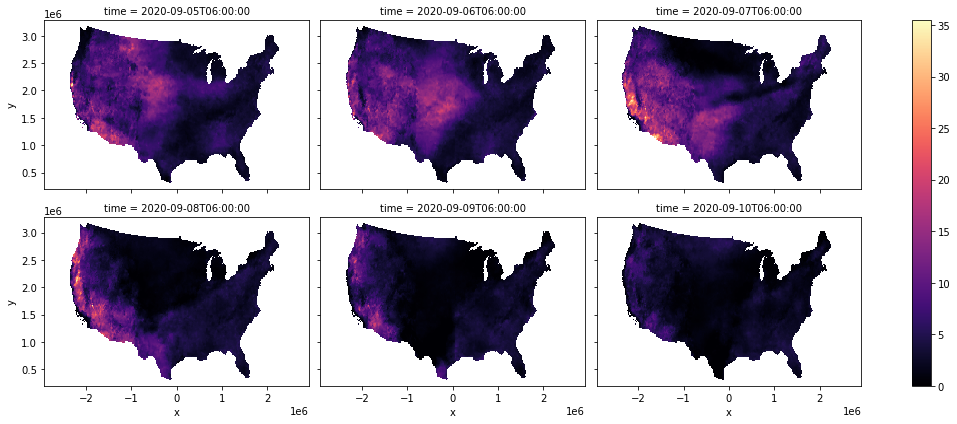
Going a little further, let’s calculate the Hot-Dry-Windy (HDW) index and see how it changed over the 6 days.
[9]:
hdw = arr.vs * arr.vpd

hdw.plot(col="time", col_wrap=3, cmap="magma", figsize=(15, 6))
[9]:
<xarray.plot.facetgrid.FacetGrid at 0x7fa51c5b0cd0>
Note
This page was auto-generated from a Jupyter notebook. For full functionality, download the notebook from Github and run it in a local Python environment.